How Do Calibrations Work?
The combination of variable depth measurement, uneven voltage distribution, and overlapping elemental peaks precludes simple analysis with X-ray fluorescence data. For these reasons, empirical calibrations are used. Empirical calibrations typically employ a variant of the Lucas-Tooth Empirical Calibration equation:
Ci = r0 + Ii(ri + Σrin+In)
Where Ci represents the concentration of element, r0 is the intercept/empirical constant for element i, ri - slope/empirical coefficient for intensity of element i, rn is the slope/empirical constant for effect of element n on element i, Ii is the net intensity of element I, and In is the net intensity of element n. This equation assumes knowledge of the variation of other elements (rn and ln in this equation; this is because some elements influence the fluorescence of others. Think of this as a much more simple equation:
y = mx + b
where x represents an independent variable, m is the slope, b is the intercept, and y is the predicted variable. In this case, think of y as the elemental concentration (in % or ppm weight) and x as the photons from your spectrum. At that point, m is just a conversion factor and b a correction. Let’s take a look at this example from the Bruker obsidian calibration:
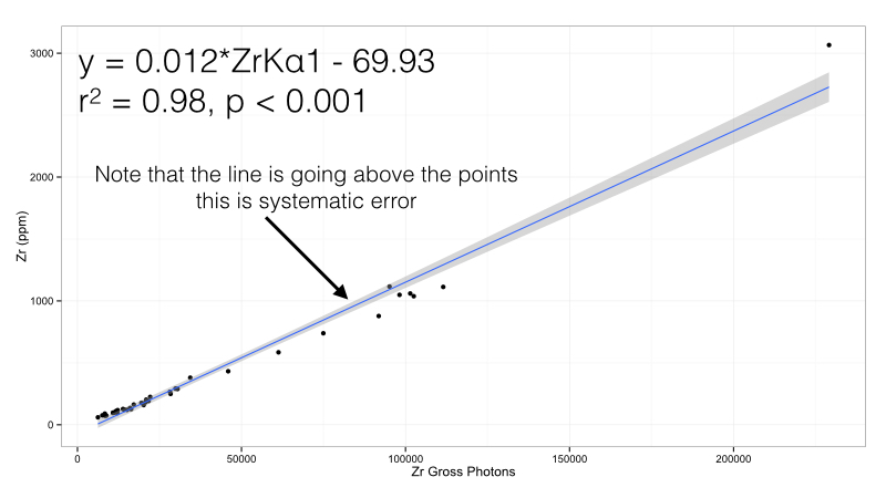
Figure 1: Zirconium calibration curve in the Bruker Obsidian calibration. Note the presence of systematic error.
In this case, there is one value (almost 3066 ppm of Zr) that has leverage over the line - it is literally pulling it up from the rest of the data. This adds systematic error - we will over estimate points from 400 - 2000 ppm Zr using this calibration formula. The benefit of this calibration curve is that it is simple, we only multiply by 0.012 and subtract 69.93 ppm to get an estimate. But this point will cause problems. There are two solutions. The first is simply to remove it:
In this case, there is one value (almost 3066 ppm of Zr) that has leverage over the line - it is literally pulling it up from the rest of the data. This adds systematic error - we will over estimate points from 400 - 2000 ppm Zr using this calibration formula. The benefit of this calibration curve is that it is simple, we only multiply by 0.012 and subtract 69.93 ppm to get an estimate. But this point will cause problems. There are two solutions. The first is simply to remove it:
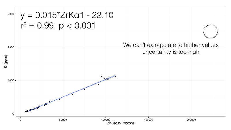
Figure 2: Zirconium calibration curve in the Bruker Obsidian calibration, high value removed
This calibration is much better - the systematic error is now gone and we are left with a simple model to quantify Zr - just multiply the photon counts by 0.015 and subtract by 22.10 ppm. But our range is more constricted - if we do get a high value we cannot simply continue the line past the maximum datapoint. The line may be accurate - but it will not be valid. We cannot quantify what we don’t know past that point. Still, if all our expected values fall between 10 and 1,000 ppm, this calibration would work well. But if we do need the expanded range, we can try a more complicated calibration curve:
This calibration is much better - the systematic error is now gone and we are left with a simple model to quantify Zr - just multiply the photon counts by 0.015 and subtract by 22.10 ppm. But our range is more constricted - if we do get a high value we cannot simply continue the line past the maximum datapoint. The line may be accurate - but it will not be valid. We cannot quantify what we don’t know past that point. Still, if all our expected values fall between 10 and 1,000 ppm, this calibration would work well. But if we do need the expanded range, we can try a more complicated calibration curve:
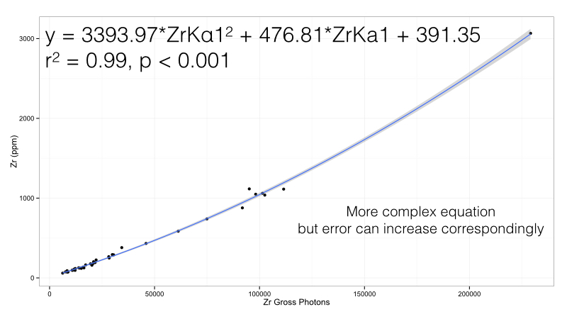
Figure 3: Zirconium calibration curve in the Bruker Obsidian calibration. Note this is a polynomial curve
Here we use a second order polynomial rather than a simple linear regression. This works very well for the range we have - there is only one potential complication. By using a more complex formula, we are exposed to more complex error. If we have unanticipated interactions with other elements, then we would have a very extreme value. In short, the more complex a calibration is, the more fragile it becomes. This becomes evident in the real world, where an almost perfect calibration becomes useless. For one element this is a challenge, but remember that we must do this for all elements:
Here we use a second order polynomial rather than a simple linear regression. This works very well for the range we have - there is only one potential complication. By using a more complex formula, we are exposed to more complex error. If we have unanticipated interactions with other elements, then we would have a very extreme value. In short, the more complex a calibration is, the more fragile it becomes. This becomes evident in the real world, where an almost perfect calibration becomes useless. For one element this is a challenge, but remember that we must do this for all elements:
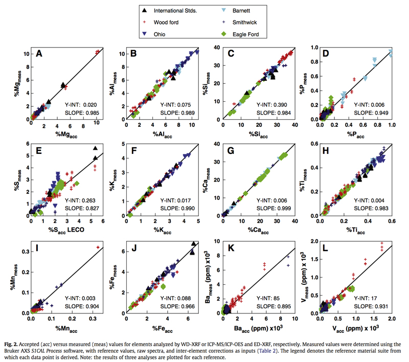
Figure 4: Calibration validation of mudrock standards (from Rowe et a. 2012).
In one critical case for obsidian sourcing, the k-alpha peak for zirconium overlaps with the k-beta peak for strontium. If a quantification procedure does not factor this overlap into its algorithms, then the reported quantity of zirconium will be influenced by the quantity of strontium. A key strength of the Lucas-Tooth algorithm is that it corrects for these effects in producing linear models for the quantification of each element. Empirical calibrations following this algorithm will be accurate within the confines of the regression line (that is to say,minimum and maximum point). Thus, the accuracy of the algorithms is contingent upon the elemental variation captured by the empirical reference set and it's appropriateness to the material being studied.
For an empirical calibration to work, a number of assumptions must be met. First, the data must be homogenous or, at the very least, sufficiently well mixed to be practically homogenous. Second, the reference set must consist of the same material. Third, every element present in the sample must also be present in the reference set. Fourth, the reference set must encapsulate the minimum and maximum of every element. In addition to these four principles, the data must be taken with the same parameters. These include the same energy, current, filter, and atmosphere (dry air, vacuum, etc.).
A calibration is necessary to translate luminescence data (e.g. photon quantities/intensities) to quantitative chemical units. A calibration has the secondary effect of reducing instrument-to instrument variation. Every instrument, even those which contain the same components, have slight variations in photon excitation and detection due to manufacturing variation in bulbs and very slight variance in internal geometries (Figure X). These differences manifest themselves in the spectra.
At this point, it is worthwhile pointing out what elements can and can’t be identified using XRF as a technique, these are determined by the energy range of photons sent out (in keV) and the resolution of the detector (in eV). Systems with a pin-diode detector (with a 185 eV FWHM resolution) can see K-alpha peaks for elements ranging from magnesium to barium and L-alpha peaks from barium to uranium when a range of 40 keV photons are detected in the sample. Systems with a silicon drift detector can include both sodium and neon as those detectors have a resolution of 144 eV at Mn Kα1. There is, however, no ED-XRF system that is able to detect oxygen directly via a K-alpha fluorescence peak. As such, only elements from sodium to uranium are currently quantifiable using XRF. This is important, as the results of XRF analysis are commonly reported in oxide form. While for a piece of obsidian it is undoubtably likely all elements detected via XRF are bound to oxygen, this is not true for all sedimentary materials, such as rocks or sediments. Many elements have multiple oxidization states. For example, FeO Fe3O4, Fe2O3 can be present in a sample. Or, hydroxide could be a possibility, Fe(OH)2. And it isn't the case that one state is predominant enough to justify the assumption that it exists exclusively in a material. FeO forms about 3.8% of oxides in continental composition, while Fe2O3 forms 2.5%. An XRF system that interprets an Fe K-alpha peak only as Fe2O3 regardless of the sample is potentially inaccurate. XRF cannot determine the molecular structure of a substance, it can only identify elements and their quantities. It is, however, possible to infer molecular structure using XRF data using correlations between K-alpha and L-alpha peaks. For example, a correlation between Ca and S could help identify calcium sulfate (CaSO4). However, it is important to note that a correlation between elements could also be indicative of a separate chemical process that selected for elements with certain properties.
In some cases, an alternative calibration approach, known as Fundamental Parameters can be employed. This approach typically relies upon iteration of data to converge upon a chemical concentration consistent with the spectra. In the case of modern metal alloys or other industrial materials this approach can be helpful because of the limited range of options and relatively predictable chemical composition. For archaeological materials that can be much more chemically diverse and variable, this approach is not appropriate. In particular, as the answer to an archaeological material can depend upon a difference of a few parts per million of a trace element (as is the case for obsidian sourcing) empirical calibration is necessary as it can be evaluated externally to determine if the method is appropriate.
While empirical calibrations can provide highly accurate results, a calibration itself adds no new information that was not already present in the X-ray fluorescence spectra - the calibration only translates the variation present in the x-ray spectra into chemical weight percents. As such, semi-quantitative analysis should be possible. One frequently used route is Bayesian Deconvolution, in which known inter-elemental effects are used in multiple resimulations of the data to produce a net photon count for each element. Other, more simple methods can be used, such as normalizing gross photon counts to either the Compton curve or valid count rate.
The Quantification and Application of Handheld Energy- Dispersive X-ray Fluorescence (ED-XRF) in Mudrock Chemostratigraphy and Geochemistry; ChemicalGeology 324- 325 (2012), 122-131; Harry Rowe, Niki Hughes, Krystin Robinson (Earth and Environmental Sciences, University of Texas at Arlington, Texas).