Using Helium
In my workshops I typically advocate controlling 5 parameters for analysis. Energy, Current, Filter, Time, and Atmosphere. Atmosphere isn't simply a matter of whether you are using vacuum or helium or not. Atmosphere, at least with handheld XRF, is every substance between your sample and your detector. This includes the Nitrogen, Oxygen, and Argon in the air, as well as the prolene that covers the nose of the instrument. Even in vacuum conditions, we are unable to always get a perfectly flush position agains the vacuum window and thus leave a little bit of air (not to mention the prolene). There are two reasons why helium may be preferable when analyzing light elements. The first is the fact that the window is gone; that 4 (or 8) micron thick prolene window does a lot to attenuate light elements. Secondly, it ensures that the photons returning from the sample have a clear path as the helium can cover almost all the distance between it and the detector.
In my workshops I typically advocate controlling 5 parameters for analysis. Energy, Current, Filter, Time, and Atmosphere. Atmosphere isn't simply a matter of whether you are using vacuum or helium or not. Atmosphere, at least with handheld XRF, is every substance between your sample and your detector. This includes the Nitrogen, Oxygen, and Argon in the air, as well as the prolene that covers the nose of the instrument. Even in vacuum conditions, we are unable to always get a perfectly flush position agains the vacuum window and thus leave a little bit of air (not to mention the prolene). There are two reasons why helium may be preferable when analyzing light elements. The first is the fact that the window is gone; that 4 (or 8) micron thick prolene window does a lot to attenuate light elements. Secondly, it ensures that the photons returning from the sample have a clear path as the helium can cover almost all the distance between it and the detector.
You will need to place the Tracer with the nose pointing down (ideally with the tripod). Then, you will need to remove the prolene window. This risk is exposing the detector to dust and the particles, but as long as it is upside down the risk is greatly minimized. I do not remove the Beryllium window for my helium analysis.
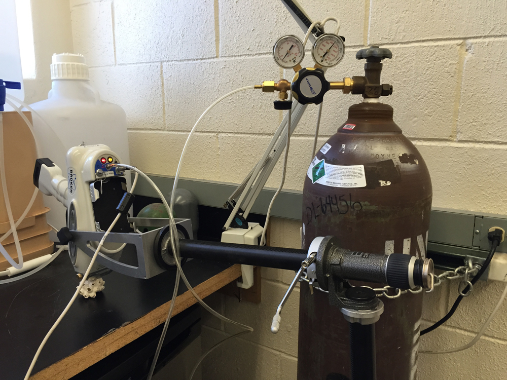
Important point - start helium flow BEFORE you connect to the Tracer. That way you protect the Tracer from any errors in regulation helium flow. The risk is that the flow is too quick and risks internal damage to the system.
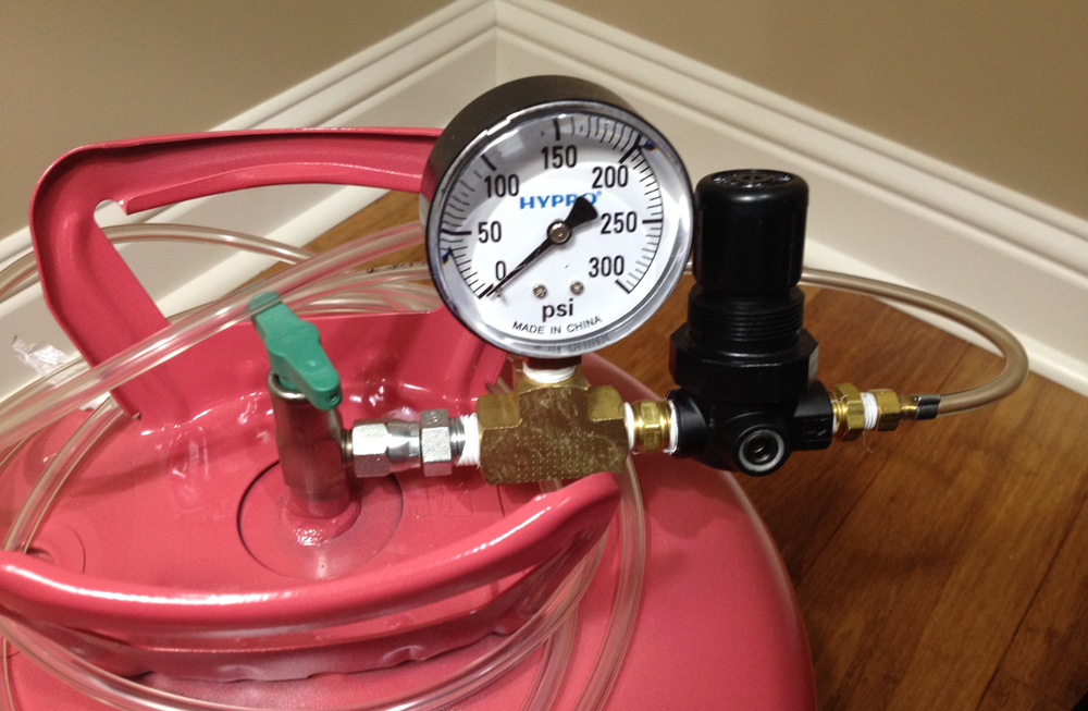
Turn on the helium tank to a heavy flow. Rely upon the regulator to throttle the flow down. This is so that the pressure on the regulator stays constant. A common error is to turn the helium tank on low with the regulator. This will work fine for a little while, but eventually the flow starts ebbing as pressure in the tank drops - this is hard to notice when you are taking many spectra. It is better to let the regulator handle the flow rate and keep the helium tank at a higher flow rate to maintain pressure. On the regulator, the flow rate you want to aim for is 0.4 LPM or less- but in reality this is a very difficult thing to attain with many regulators as your indicator will essentially be resting on 0. It is better to go by feel. Turn the regulator down low enough so that you can barely hear it and barely feel it brush against your cheek.
Important point - start helium flow BEFORE you connect to the Tracer. That way you protect the Tracer from any errors in regulation helium flow. The risk is that the flow is too quick and risks internal damage to the system.
Turn on the helium tank to a heavy flow. Rely upon the regulator to throttle the flow down. This is so that the pressure on the regulator stays constant. A common error is to turn the helium tank on low with the regulator. This will work fine for a little while, but eventually the flow starts ebbing as pressure in the tank drops - this is hard to notice when you are taking many spectra. It is better to let the regulator handle the flow rate and keep the helium tank at a higher flow rate to maintain pressure. On the regulator, the flow rate you want to aim for is 0.4 LPM or less- but in reality this is a very difficult thing to attain with many regulators as your indicator will essentially be resting on 0. It is better to go by feel. Turn the regulator down low enough so that you can barely hear it and barely feel it brush against your cheek.
Following this, plug the tube into the Tracer. If the 8 mm tube does not fit right, you will need to wrap the teflon tape around the vacuum nozzle of the Tracer. Do not use the standard brass vacuum plug - this will block the flow. Aim for an open tube that fits over the vacuum port nozzle. Once you’ve done this, you can put your finger below the nose of the Tracer to gently feel the cool helium blowing through.
Once this is done, lower the Tracer onto the sample you want to measure, leaving about half of 1 mm gap between the sample and the nose to allow helium to escape. Then, you can take your measurement. I recommend 15 keV, 25 μA, and no filter. I’ve had good success running analysis for about 180 seconds. Below is a comparison of sample BL-122 taken with both vacuum (green) and helium (red). The assay time was 240 seconds with helium, 300 seconds with vacuum.
Once this is done, lower the Tracer onto the sample you want to measure, leaving about half of 1 mm gap between the sample and the nose to allow helium to escape. Then, you can take your measurement. I recommend 15 keV, 25 μA, and no filter. I’ve had good success running analysis for about 180 seconds. Below is a comparison of sample BL-122 taken with both vacuum (green) and helium (red). The assay time was 240 seconds with helium, 300 seconds with vacuum.
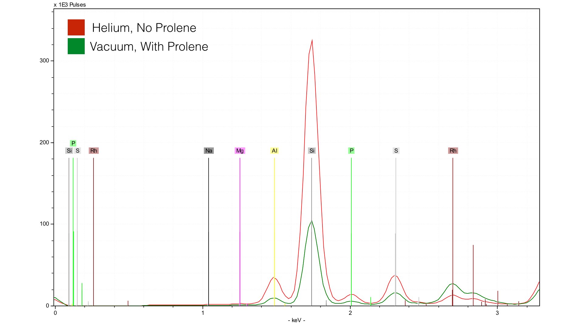
You can see much higher concentrations of Si and Al due to the helium purge. Note, however, that the compton and raleigh scattering around the Rh L-line (~2.5 keV) is much higher for the spectra from the vacuum - this will become important when we talk about quantification. Let's take a closer look at our light elements, specifically Mg and Na. In BL-122, both Mg and Na are at ~0.7%
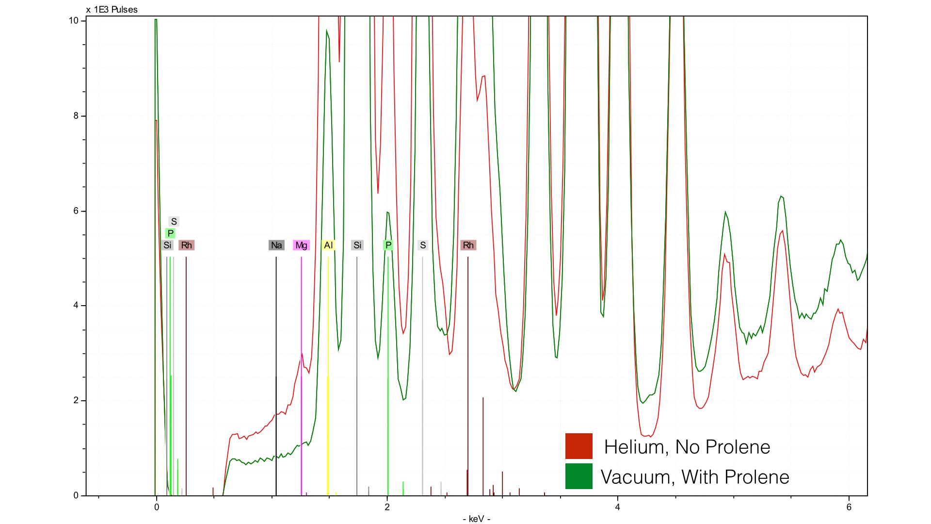
You can see Mg is much better defined, and Na is even a little visible, though very much at the limit of detection. Clearly, for Mg, helium provides much better signal to noise. However, in creating this calibration I found a major problem - there was no improvement in error. For the mudrock reference set, measured at 300 seconds with a vacuum the average difference (reported in S1CalProcess) was 0.34%. For the data taken with helium at 240 seconds, the error was 0.33%. Not exactly an earth shattering difference. The problem, as it turns out, is normalization. Things change with helium. First though, lets look at the reference spectra taken with the vacuum.
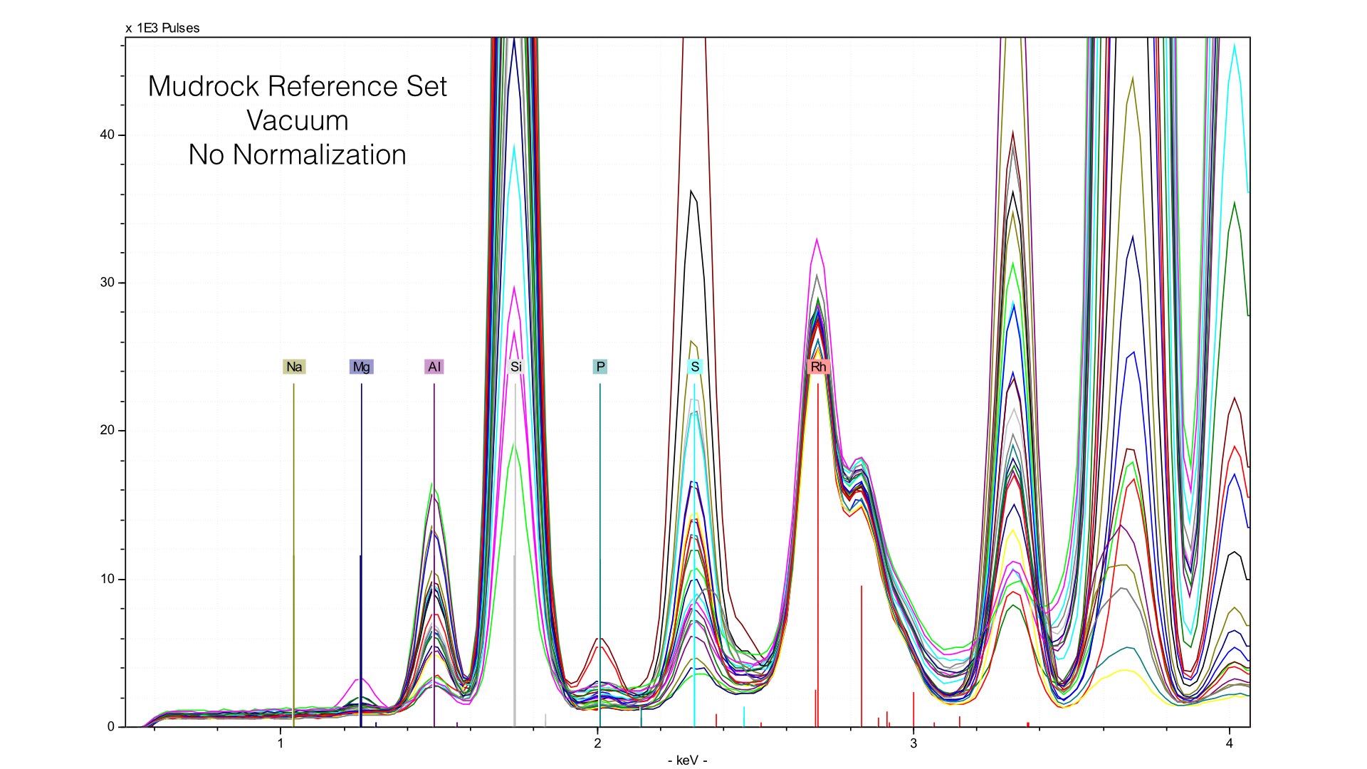
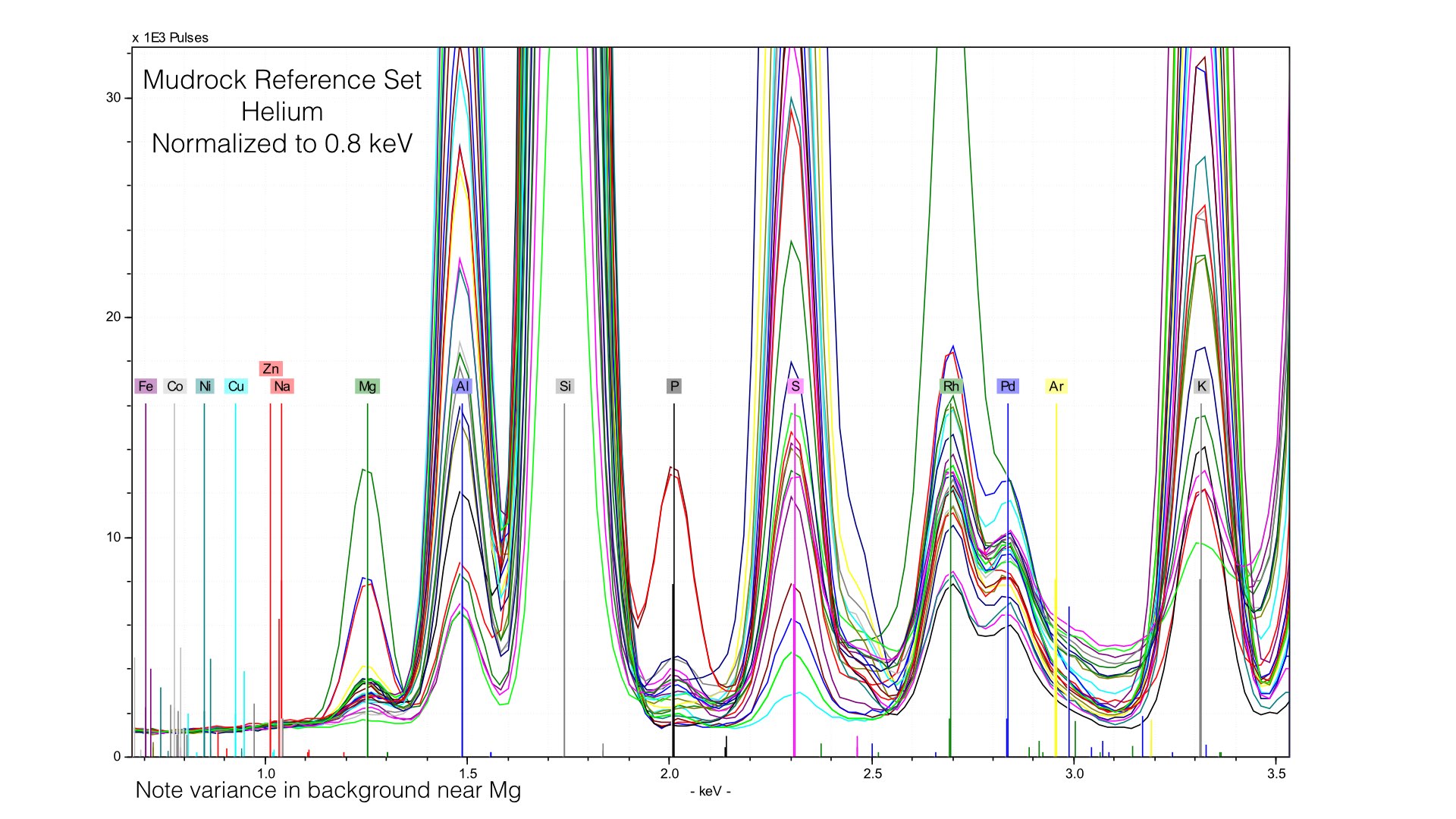
Typically, we normalize from 2.8 to 3.1 keV in the mudrock cal. You can see how this affects the spectra in the following image:
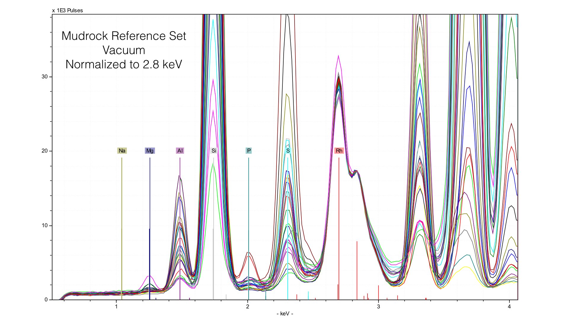
Normalizing the spectra is a critical step in quantification, and here it is well done. You can observe a common baseline for each light element. Here, you can see the range of Magnesium. The maximum value (highest peak) is ~10 weight %. Now let's take a look at what happens when we remove the prolene window and take spectra of the same reference samples.
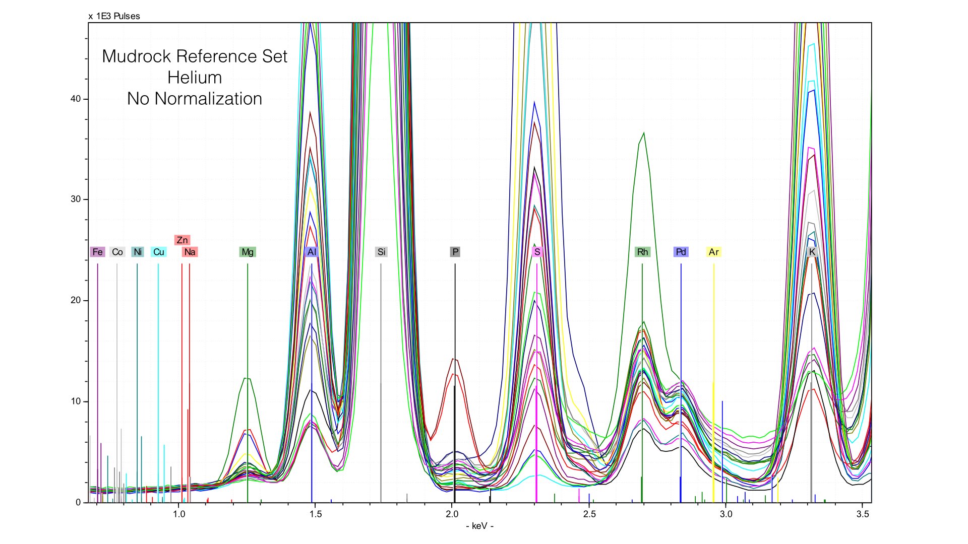
Here, you can see two things. First, the height of the Rhodium L-line is much smaller relative to nearby elements like Sulfur. Second, it is much more variable. If we follow the same normalization protocols as we did with our data taken in vacuum conditions, we end up with very distorted peaks:
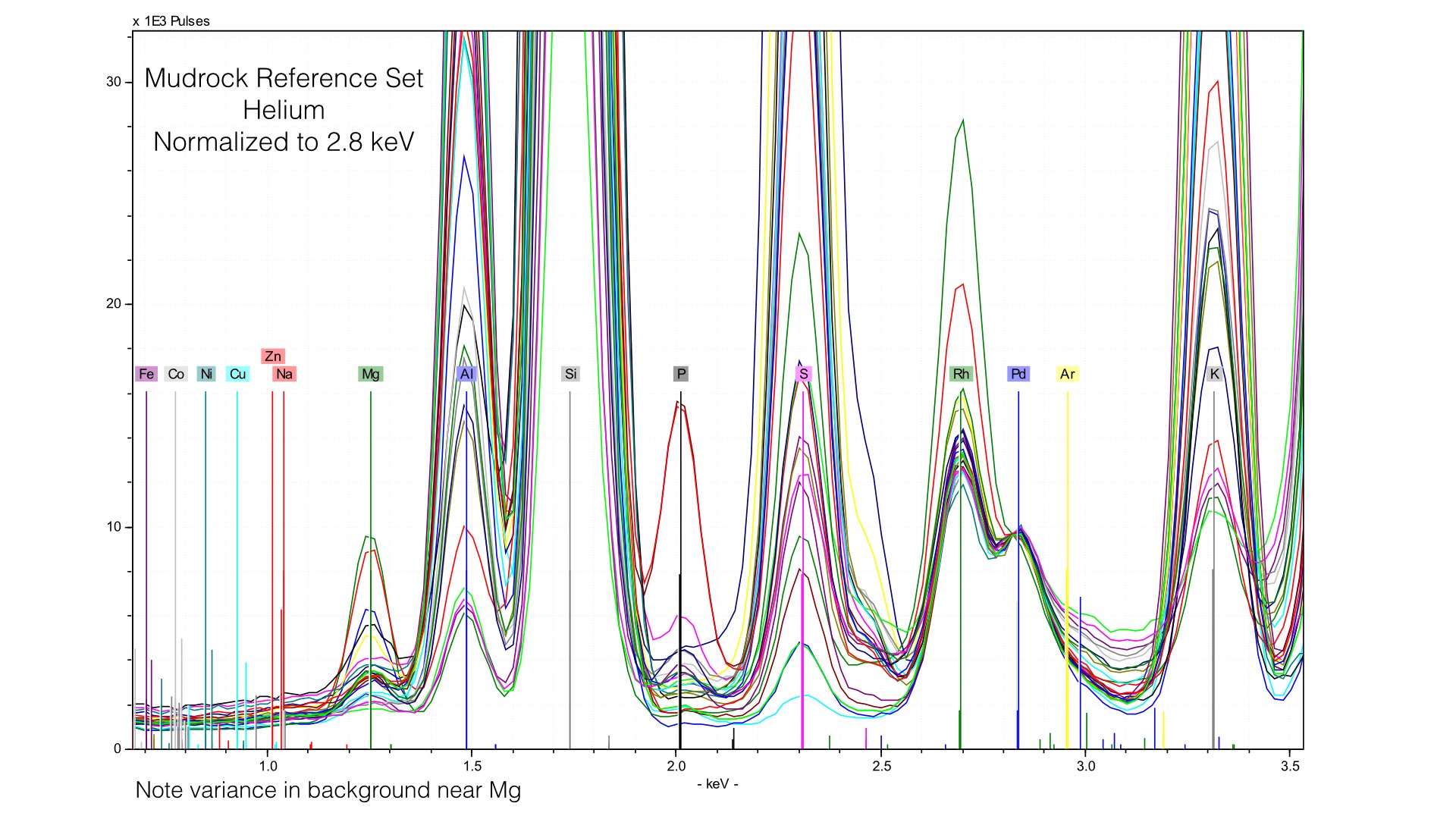
The problem here is that our 4 μm prolene window was providing much of the Rhodium L-line scatter. Removing it creates a smaller, but more variable peak. We are more exposed to the variation in the electron cloud of the matrix, and this generates effectively a new data source. Normalizing to this makes as much sense as normalizing to an elemental peak. It also provides an important lesson - our light element normalization is actually normalizing to the prolene window, not the sample. That is fine, but it is important to note that your light element calibrations will be sensitive to any changes in that window when it is present. If we zoom into Magnesium, we can see that this is pretty mucheradicating any gain in helium. Sure enough, our average difference in Magnesium concentrations is 0.32% here, compared to 0.34% earlier. If we instead normalize at a different point of the spectrum though, things look quite different.
Here, I normalized the spectra between 0.7 and 0.9 keV, and the baseline for light elements is much improved. This also produces better quantification results, the average difference in Magnesium goes down from 0.32% to around 0.10%. But this comes at the cost of acuracy in heavier elements - Potassium or Calcium will have a worse baseline if we normalize at such a low energy. The key point here is that if you use Helium, you will need to produce multiple calibration files with different normalization stop see the ill improvement in your data. I typically create two, one for Sodium through Sulfur, and a second for Potassium to Iron.
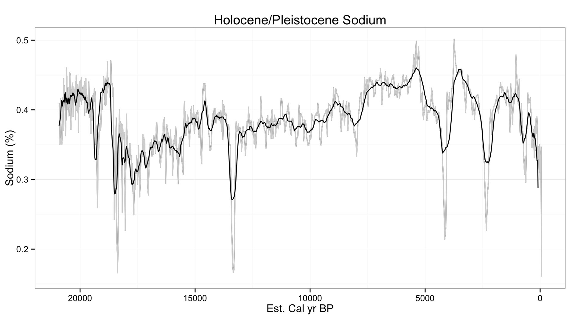
Finally, let's take a look at a different set of data to see just how low we can go with Sodium using a geologic core. The core goes back at least 20,000 years, but they are still revising the age model. In any case, here is Sodium from that core.
Finally, let's take a look at a different set of data to see just how low we can go with Sodium using a geologic core. The core goes back at least 20,000 years, but they are still revising the age model. In any case, here is Sodium from that core.
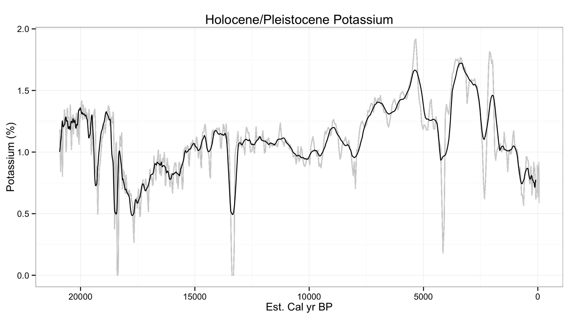
Variation in Sodium occurs between 0.5 to 0.2 weight %, a surprisingly (and suspiciously) low value. This is quite lower than the minimum detection limit I have told many of you (~0.7 %). I checked Potassium to see its variation, and it looks similar.
Both Sodium and Potassium are class 1 elements, they tend to vary together. So it follows that we use variation in Potassium as a test to see our relationship with Sodium. Here is a simple bivariate scatterplot with Sodium on the x axis and Potassium on the y.
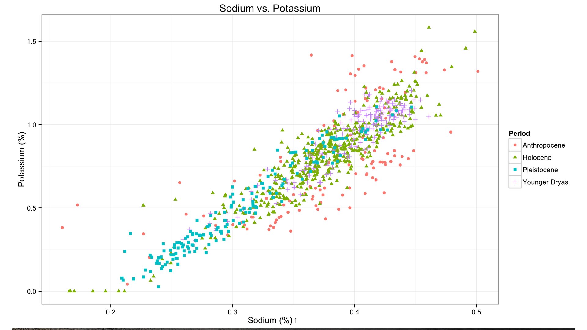
As you can see, we have a statistically significant correlation between the two. This suggests we are indeed measuring Sodium at quite low concentrations in this core. The relationship breaks down at around 0.23%.
As has been said before in this thread, the sensitivity to Sodium will vary from matrix to matrix, and sample heterogeneity will always be a concern. But the core lessons are as follows:
1. Flow helium through the vacuum port, use a minimal flow.
2. Use region-specific normalization for very light elements.