Normalization
What color is this dress?
What color is this dress?

It will either be blue and black or white and gold. If you haven’t seen it before, you’re probably surprised to hear that anyone would see it any other way - it is obviously white and gold/blue and black.
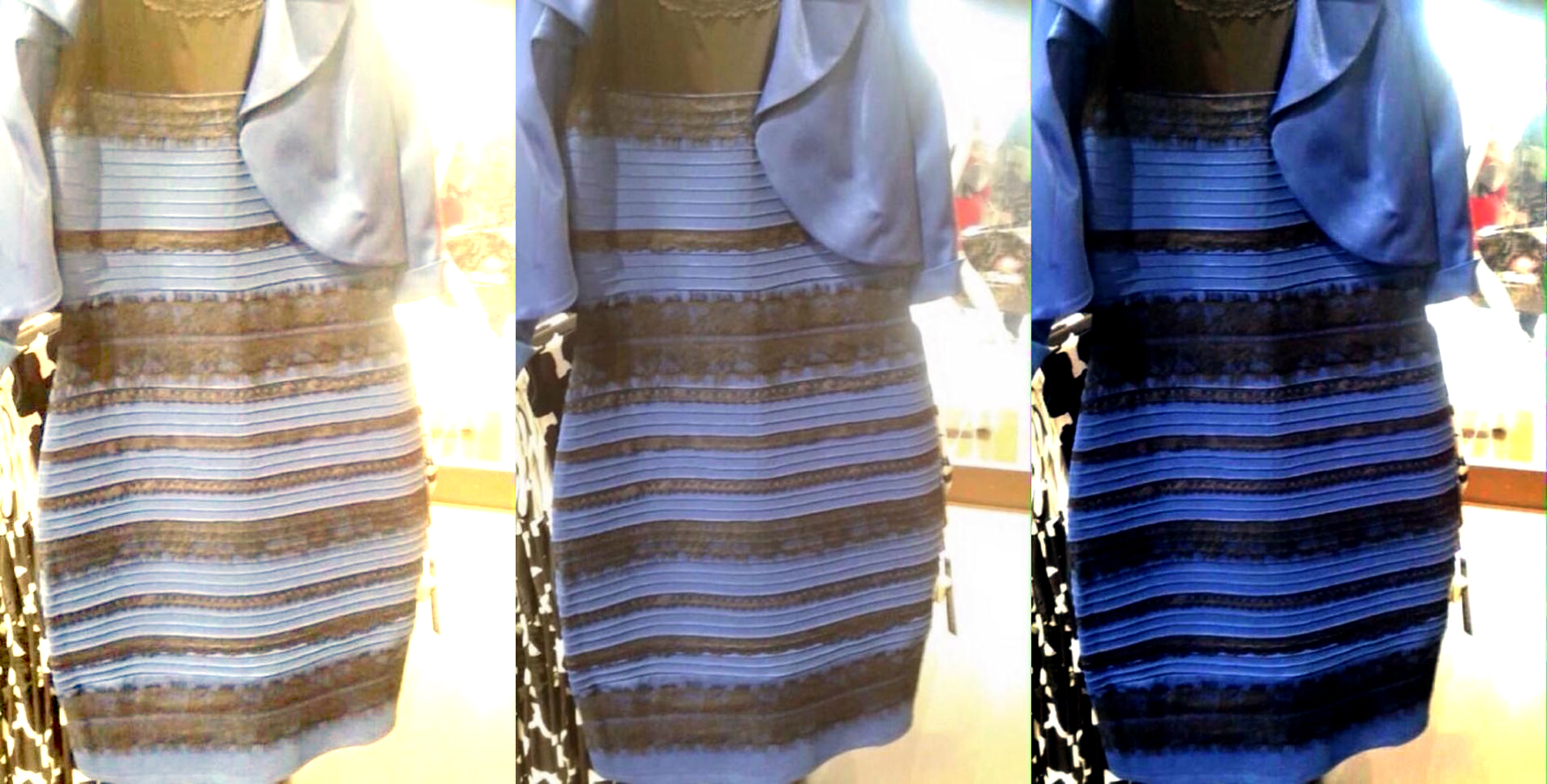
The perception of the dress is not a problem with your eyes - those who see the blue and black dress (or white and gold dress) have the same cone cells as you do. The problem is with your brain - it will choose a native white point in the photo and once it has done that, everything else will follow. For example, if you see a blue and black dress, you have normalized the white point to the lower right hand corner of the photo. If, however, you see a white and gold dress, your mind will pick the stripes in the dress and ‘make’ those white. The gold then follows from there. In other words, the phenomenon is one of normalization. How you normalize data can completely transform it. This is true of XRF spectra as well. Take a look at the following spectra from silicates.
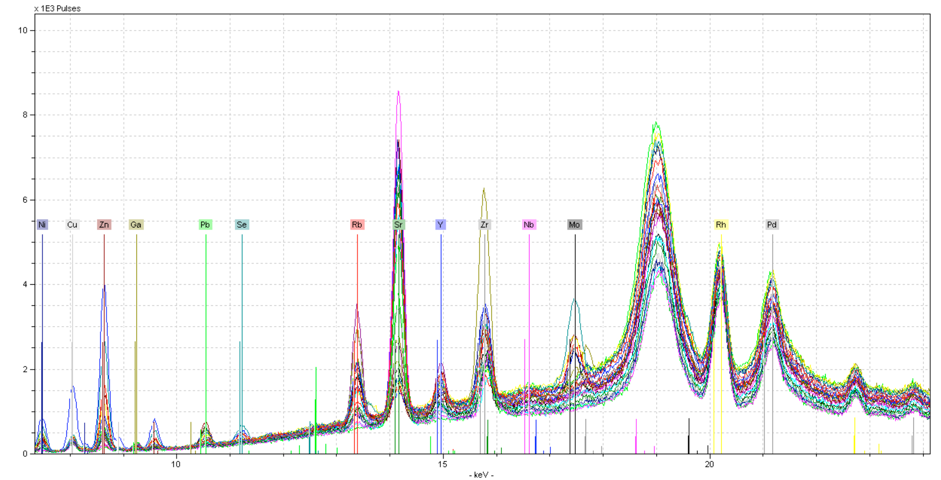
Here you can see lots of noise in the spectra - this is because a silicate is primarily made of Oxygen. Large changes in the Oxygen and/or Carbon content can result in more background scatter as photons bounce around the sample. This can be corrected to some degree by normalizing to a portion of the background scatter. In this case, we will normalize to the Compton peak (18.5 - 19.5 keV), this is the inelastic scatter from the Rhodium tube.
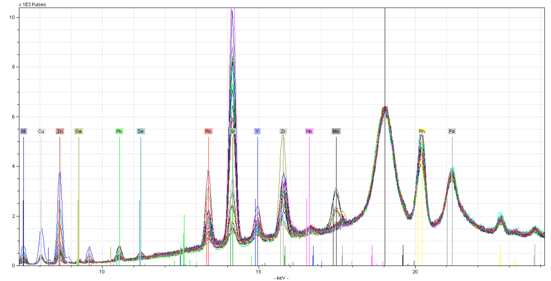
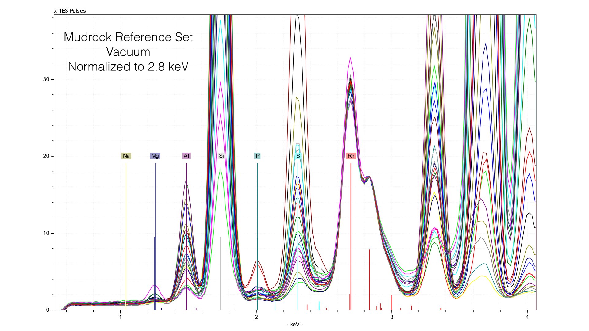
Now, all elements share a common baseline, and qualitative analysis is easier. In fact, quantitative analysis will also improve with this kind of normalization. With spectra like this, normalizing at the Compton peak is often the standard. But when we analyze lighter elements, this can become more of a challenge. Take the following spectra taken at 15 keV under vacuum conditions:
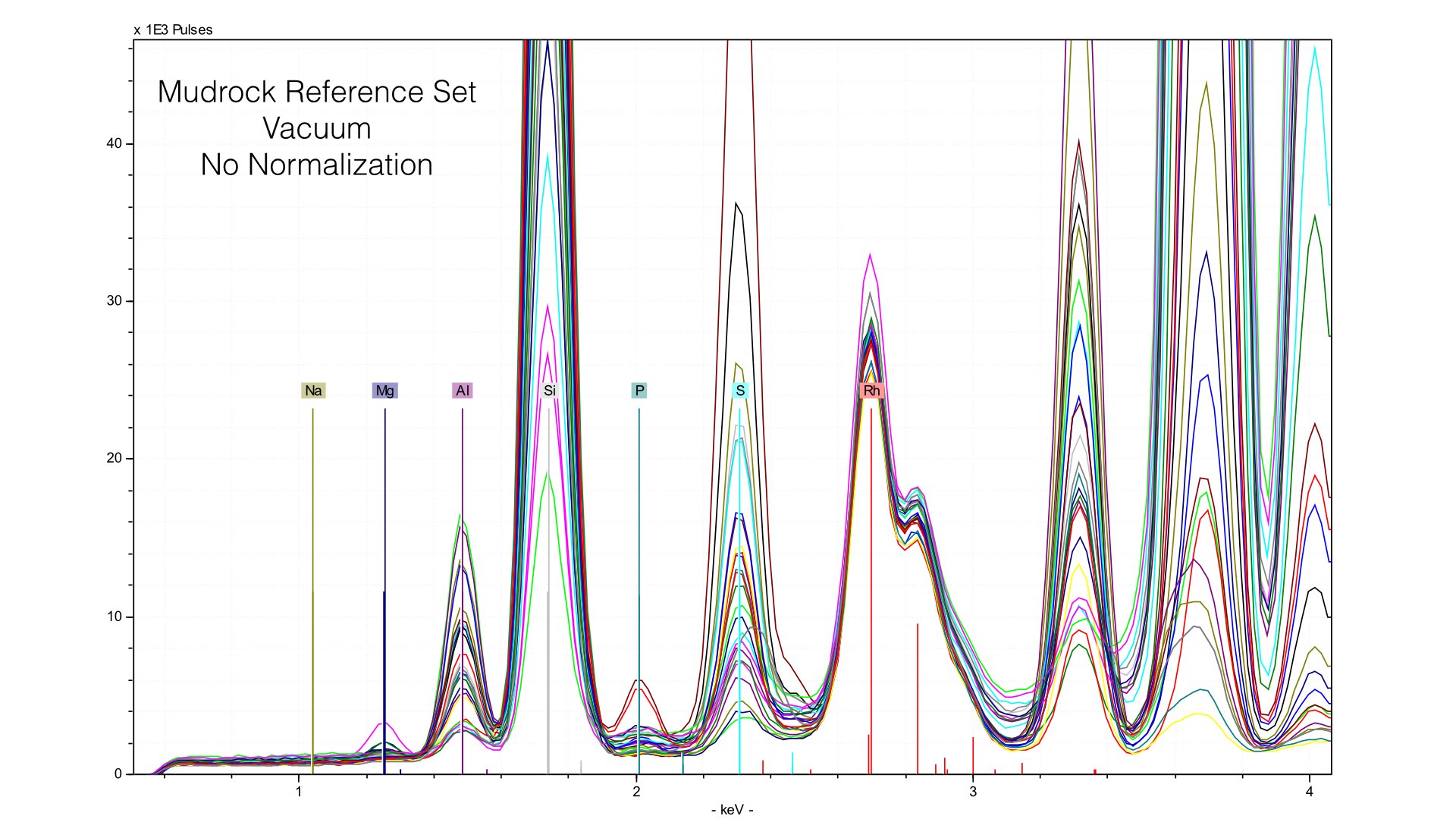
Typically, we normalize from 2.8 to 3.1 keV in the mudrock cal. You can see how this affects the spectra in the following image:
Normalizing the spectra is a critical step in quantification, and here it is well done. You can observe a common baseline for each light element. Here, you can see the range of Magnesium. The maximum value (highest peak) is ~10 weight %. Now let's take a look at what happens when we remove the prolene window and take spectra of the same reference samples.
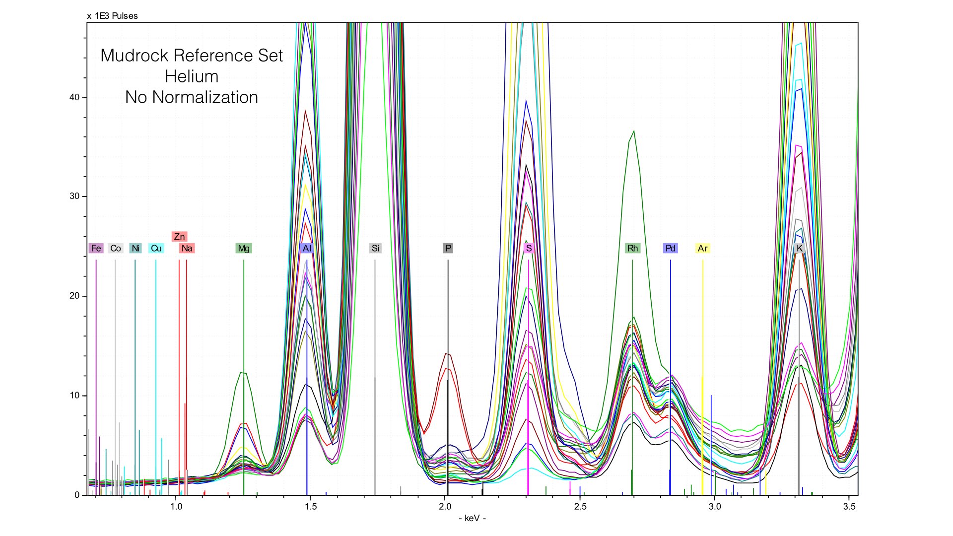
Here, you can see two things. First, the height of the Rhodium L-line is much smaller relative to nearby elements like Sulfur. Second, it is much more variable. If we follow the same normalization protocols as we did with our data taken in vacuum conditions, we end up with very distorted peaks:
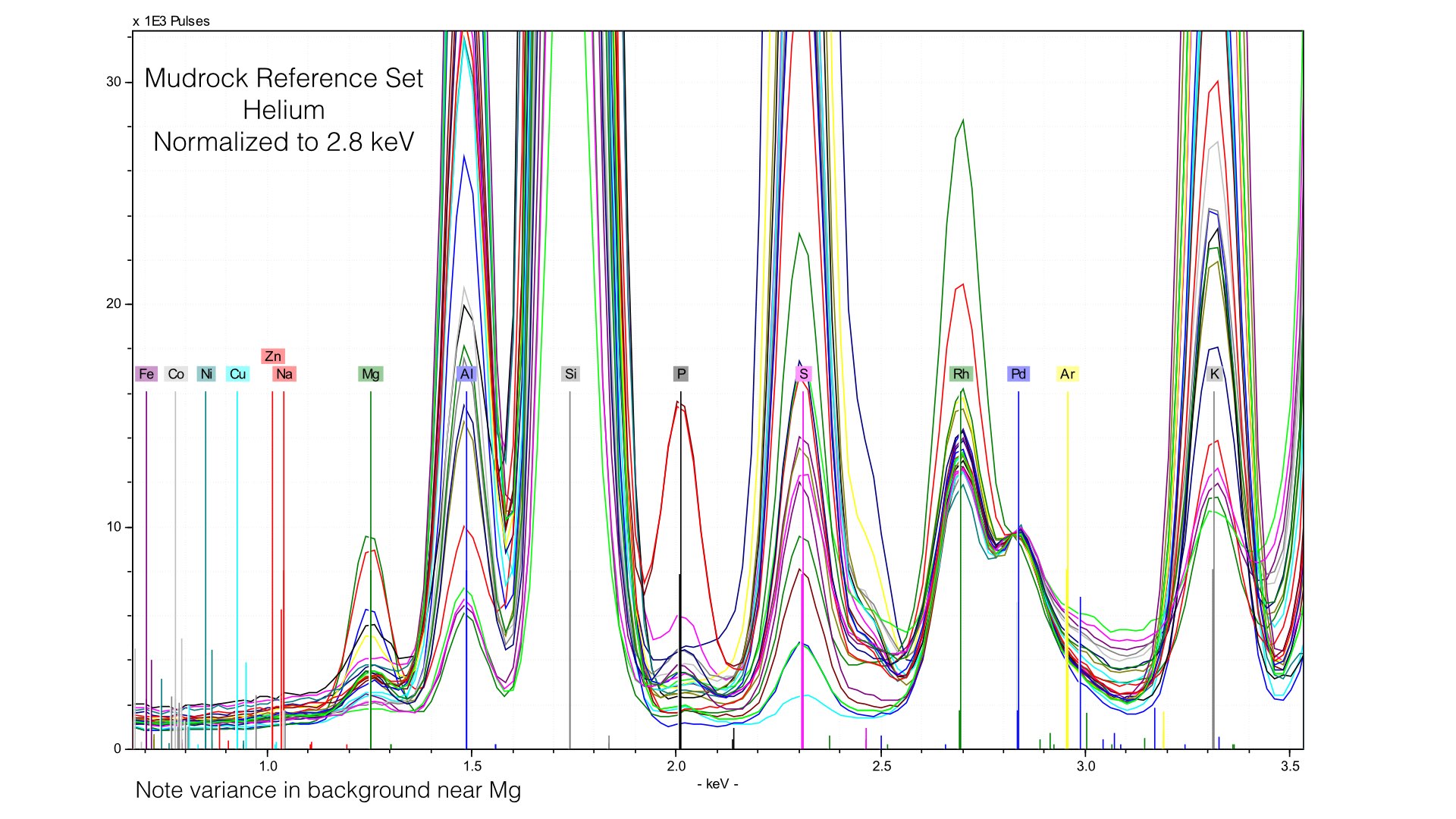
The problem here is that our 4 μm prolene window was providing much of the Rhodium L-line scatter. Removing it creates a smaller, but more variable peak. We are more exposed to the variation in the electron cloud of the matrix, and this generates effectively a new data source. Normalizing to this makes as much sense as normalizing to an elemental peak. It also provides an important lesson - our light element normalization is actually normalizing to the prolene window, not the sample. That is fine, but it is important to note that your light element calibrations will be sensitive to any changes in that window when it is present. If we zoom into Magnesium, we can see that this is pretty mucheradicating any gain in helium. Sure enough, our average difference in Magnesium concentrations is 0.32% here, compared to 0.34% earlier. If we instead normalize at a different point of the spectrum though, things look quite different.
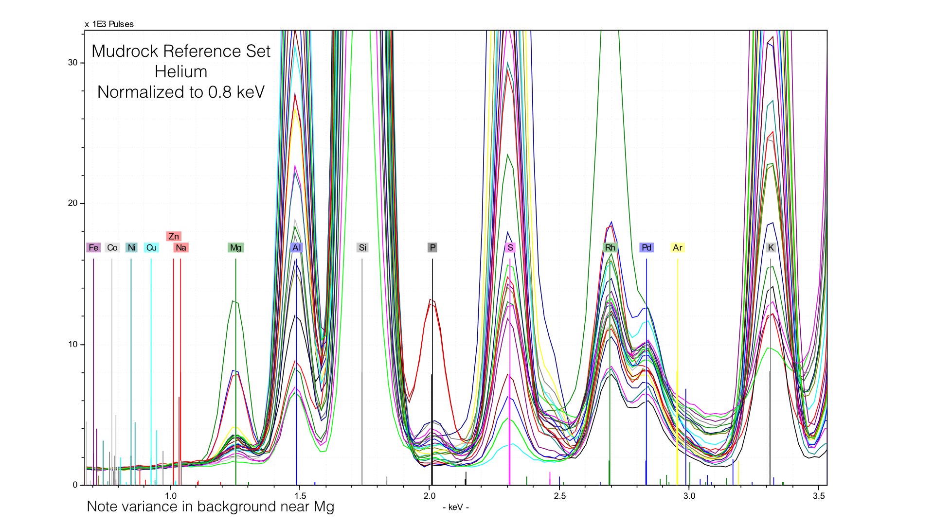
Here, I normalized the spectra between 0.7 and 0.9 keV, and the baseline for light elements is much improved. This also produces better quantification results, the average difference in Magnesium goes down from 0.32% to around 0.10%. But this comes at the cost of acuracy in heavier elements - Potassium or Calcium will have a worse baseline if we normalize at such a low energy. The key point here is that if you use Helium, you will need to produce multiple calibration files with different normalization stop see the ill improvement in your data. I typically create two, one for Sodium through Sulfur, and a second for Potassium to Iron.